Metrics and Fact Tables
Metrics are how you measure success and failure for your business. An e-commerce company might have metrics related to conversion rates, revenue, and cart abandonment. A B2B SaaS company might have metrics around subscription trials, cancellations, and usage. Every company is different and GrowthBook is flexible enough to support a wide variety of use cases.
The primary way to create metrics in GrowthBook is with Fact Tables where you write SQL to pull a set of rows and then define multiple metrics on top of those rows. There is also a legacy method where each metric has its own self-contained SQL. Fact Tables are easier to use, faster to query, and more powerful, so we highly recommend using them for all new metrics.
If you learn best by example, you can jump straight into Metric Examples and Use Cases.
Fact Tables
Fact Tables are defined by a SQL SELECT statement and are the base that metrics are built on top of.
At a minimum, a Fact Table must select the following columns:
timestamp- The date the event happened- One column per supported identifier type (e.g.
user_idandanonymous_id). The possible identifier types depend on your data source settings.
Any other columns you return can be used to create metrics or used as a filter.
Here's a full example:
SELECT
  -- Required columns
  purchase_date as timestamp,
  user_id,
  anonymous_id,
  -- Additional columns (depends on your use case)
  amount,
  coupon_code,
  device_type
FROM
  orders
WHERE
  status = 'completed'
This is an example of a "modeled table", which represents a specific order event and has dedicated columns related to orders. GrowthBook also works great with raw event stream tables and even some pre-aggregated tables. Check out Metric Examples and Use Cases for more info and examples of these different data schemas and table types.
Columns
When you create a Fact Table, we query the first few rows and inspect the returned data to determine which columns you've selected and what data types they are.
This process isn't perfect. For example, if the first few rows happen to have null as the value of a column, we can't tell if it's supposed to be a number, string, etc.. When this happens, we will show you a warning and you can manually specify the type.
Number Formats
For numeric columns, you can also specify a number format, which controls how the metric is displayed on the front-end. Possible values are currency, time:seconds, memory:bytes, and memory:kilobytes.
The default display currency is USD, but you can change it under Settings → General → Metric Settings
Metric Types
There are 6 types of metrics you can create within GrowthBook - Proportion, Retention, Daily Participation, Mean, Ratio, and Quantile.
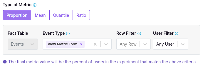
Proportion Metrics
Proportion Metrics measure the percent of users in an experiment who exist in a Fact Table (and match any filters you specify).
For example, if you have an Orders Fact Table, you can create a Proportion Metric to see what percent of users purchased something. For this metric, we don't care how many times they purchased, just that they have at least 1 matching row.
Retention Metrics
Retention Metrics are used to measure the retention of users over time with respect to their first experiment exposure. For example, you might want to measure the retention of users who came back to your site at least 7 days after their first experiment exposure.
You can use the filters to determine if a user qualifies as retained (using a row filter to only look for certain events or using a user filter to only look for users who completed an action a certain number of times).
You then set the retention window, which is the amount of time after the first experiment exposure that a user must do the qualifying actions. You can also use a conversion window to only look for a certain time period after the start of the retention window. For example, if you want to measure the retention of users who came back to your site in the second full week after the experiment exposure, you would set the retention window to 7 days and the conversion window to 7 days.
Daily Participation Metrics
Daily Participation Metrics measure the average percentage of days after experiment exposure that a user is active (i.e., meets the metric criteria). This is analogous to Daily Active Users (DAU) in an experiment context, where you want to measure engagement frequency over time.
For each user, GrowthBook:
- Counts the number of distinct days they match the metric criteria (have rows in the Fact Table that meet your filters)
- Calculates the number of eligible days since their first experiment exposure (based on the metric window settings)
- Computes the user's participation rate as:
(matching days) / (eligible days) - Averages these participation rates across all users in the variation
The result is displayed as a percentage (0-100%), representing the average daily participation rate for users in that variation.
Example:
If your control variation has two users:
- User 1: Meets the active criteria on 2 days and has been in the experiment for 5 days → participation rate = 2/5 = 0.4 (40%)
- User 2: Meets the active criteria on 3 out of 3 days → participation rate = 3/3 = 1.0 (100%)
The variation average would be: (0.4 + 1.0) / 2 = 0.7, or 70%. This means the average daily participation rate is 70% for users in this variation.
If you had a conversion or lookback window, the number of eligible days would be limited to the number of days in that window and the participation rate would be calculated based only on that window.
Use Cases:
- Measuring user engagement frequency (e.g., "What percentage of days do users log in?")
- Tracking feature adoption over time (e.g., "What percentage of days do users use the new feature?")
Mean Metrics
Mean Metrics are useful when there are more than 2 possible states a user can be in. For example, instead of just purchase/not purchase, you might care about the average number of orders a user makes, the average revenue you earned per user in an experiment, or a count of the distinct types of items a user purchased.
For the metric value, there are 4 types of aggregations you can do:
COUNT(*)- a count of all rows per user in your Fact TableCOUNT(DISTINCT DATE(timestamp))- the distinct number of days user completed the qualifying actions in your fact table (e.g. for a count of active days per user, akin to daily active users [DAU] metrics)SUM(column)- the sum per user of any numeric column in your Fact TableMAX(column)- the max of a numeric column per user in your Fact TableCOUNT(DISTINCT column)- the distinct count of a string column per user in your Fact Table.
Note: for COUNT(DISTINCT column) where you pass an arbitrary column, we use the HyperLogLog estimation method to approximate the distinct count while scaling to account for data with many rows and easily allow re-aggregation. However, COUNT DISTINCT is still more computationally costly than other aggregation types, so use it only when necessary. This aggregation is not available for SQL Server, MySQL, Postgres, or Vertica.
For example, an Orders per User metric would use COUNT(*) since you want to count the total number of rows. A Revenue per User metric would use SUM and select the column where the order total is stored.
The denominator for Mean Metrics is always the number of users in an experiment variation. So, even though you may be doing SUM(revenue) as the aggregation, it will be divided by number of users and you will actually end up with an average value per user, not an overall sum for the variation.
Ratio Metrics
Ratio Metrics let you pick a custom denominator and allow for metrics such as Average Order Value (denominator is number of orders) or Session Duration (denominator is number of sessions).
For both the numerator and denominator, you can select a Fact Table, an aggregation, and optional filters. GrowthBook allows the numerator and denominator to have different Fact Tables, which can open up some really advanced use cases.
The types of aggregations supported for ratio metrics are:
COUNT(*)- Number of rows in the Fact TableCOUNT(DISTINCT 'User Identifier')- Sample size of the experiment variationSUM(column)- Total of a numeric column in the Fact TableMAX(column)- Max of a numeric column in the Fact Table by userCOUNT(DISTINCT column)- Distinct count of a string column in the Fact Table by user
Under the hood, GrowthBook uses the Delta Method to accurately determine the variance.
For example, to create a Session Duration metric, you would do the following:
- Numerator:
SUM(duration)from aSessionsfact table - Denominator:
COUNT(*)from aSessionsfact table
Quantile Metrics
Quantile Metrics are useful when you care about comparing variations at a quantile (e.g. latency at P99) rather than the mean. These are also called percentile metrics. Learn more about when to use Quantile Metrics here.
One key consideration is Group by Experiment User before taking quantile?. In short, if you often think about your metric at the user level, you should aggregate. If you think about your metric at the event level, do not aggregate.
For the metric value, the only aggregation available is SUM(column). For SUM, you will be able to choose any numeric column in your Fact Table.
You have the option to Ignore Zeros.
For event-level analysis, ignoring zeros entails removing all events from the analysis with value equal to 0. Similarly, for a user-level analysis, removing zeros entails removing all rows corresponding to user-level aggregations that have value 0.
When picking Quantile you have several default options or can select Custom. If you select Custom you must input a number between 0 and 1. For example, inputting 0.75 will compare the percentiles across variations.
Filters
The real power of Fact Tables comes with filtering. This allows you to easily create metric variants.
There are 2 kinds of filtering available
- Row Filters
- User Filters
Row Filters
Row Filters determine which rows of the Fact Table are included in the metric calculation. You can define multiple Row Filters and they will be ANDed together.
Row Filters support a wide variety of operators:
=!=><>=<=innot_inis_nullnot_nullis_trueis_falsecontainsnot_containsstarts_withends_withsql_expr(raw SQL for advanced use cases)saved_filter(a saved SQL expression that can be reused across metrics)
Auto Prompting for Row Filters
It's common to have an important "type" column that you use to build out metrics. For example, if your Fact Table is a raw event stream, there will be a column like event_type to differentiate between a page view, button click, purchase, etc.. You will almost always want to filter metrics using this column.
After creating your Fact Table, you can edit a column and check the “Prompt all metrics” box. This helps GrowthBook better streamline the UI when creating metrics.
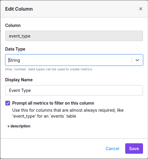
When you check this box, GrowthBook will run a quick query looking for the top 100 values for this column in the past week. This will be used to add an auto-complete field in the UI when creating a metric:
Another example use of this checkbox is for a Page Path column in a Page Views Fact Table. This will streamline creation of metrics such as "Visited /checkout", "Visited /pricing", and more.
User Filters
User Filters are applied AFTER aggregating by user. Instead of filtering individual rows, you are filtering the total value per user.
You can either filter on the Count of Rows or the SUM of a numeric column. This can be easier to understand with examples:
- Count of rows:
>= 3: Only include users with at least 3 rows in a Fact Table - SUM of a revenue column:
> 100: Only include users who have spent at least $100 total across all of their orders.
Only simple SQL comparison operators are supported: <, >, <=, >=, =, <>. User Filters can only be applied to Proportion metrics and the numerator of Ratio metrics (only when using COUNT(DISTINCT 'User Identifier')).
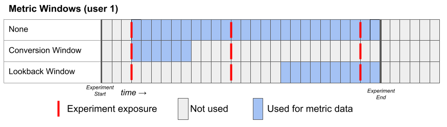
Metric Windows
When used in an experiment, we only consider rows of a Metric where the timestamp is greater than or equal to the first time the user was exposed to the experiment. In other words, if someone purchases something before seeing your experiment, it won't be included in the analysis. This behavior is ideal for the vast majority of metrics, but you can change it with the Metric Delay setting if desired (see below).
There are three window settings one can use to configure the metric date window. Each of them defines the lower and upper date range of the metric to use for each user:
- None (default for Fact Metrics)
- Lower bound: user's first exposure plus the metric delay
- Upper bound: experiment end date
- Conversion Window (default for Legacy Metrics)
- Lower bound: user's first exposure plus the metric delay
- Upper bound: the lower bound + the length of the conversion window
- Lookback Window
- Lower bound: the experiment end date minus the lookback window OR the user's first exposure plus the metric delay, whichever is later
- Upper bound: experiment end date
Here's a graphical representation of these three window types for a hypothetical User 1:
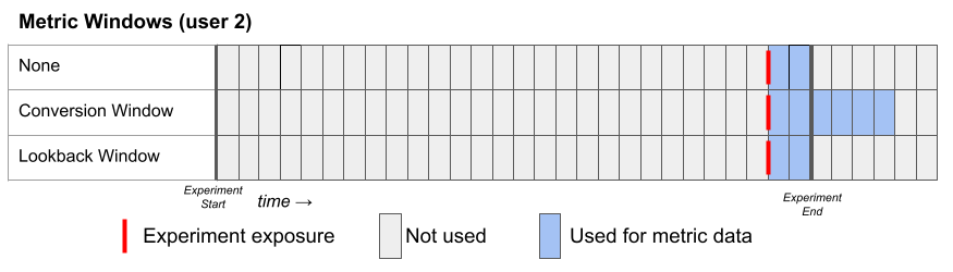
Here's a second example for a hypothetical User 2, who joins the experiment late. Notice that the conversion window can extend beyond the experiment end date.
Why might you choose one window over another?
None - The simplest. Use all data available. This is useful for using as much data associated with users in your experiment and will combine any behavior that is right after experiment exposure as well as long run behavior within the experiment time frame.
Conversion window - Conversion windows allow you to only look at events that are tied to the first exposure to an experiment. This can help if, for example, you are tracking purchases and you only want to measure the effect of an experiment in a checkout flow on purchases made soon after seeing that checkout flow. Using a conversion window can reduce the noise from user behavior not related to an experiment. However, if you set the window too short, you may not capture users that return a few days later and were influenced by the experiment.
Lookback window - Lookback windows are good for capturing long run impacts of an experiment on regular behavior like user log ins or page views. They have two main advantages:
(1) You can mitigate the novelty effect of an experiment; if you are testing a new recommendation algorithm, at first users may react a certain way to the experiment, but eventually they may adjust and so may their behavior. In these cases, you may just want to look at the last 14 days of an experiment.
(2) Lookback windows help you focus on the long run effects of an experiment. Much of experimentation is about building a better product; by focusing on impact of an experiment after it has been live for a week or two, you may get a better picture of the long run impact of launching the experiment.
Larger companies who measure long run logged in behavior want to ensure their experiments have lasting effects and often rely on lookback windows to make shipping decisions. However, lookback windows may not be right if you are testing a feature on logged-out or anonymous users and are measuring simple purchase conversions or something similar. In these cases, you might end up with many logged-out users who, in the long run, simply have no metric data associated with them.
Advanced Settings
What is the Goal?
For the vast majority of metrics, the goal is to increase the value. But for some metrics like "Bounce Rate" and "Page Load Time", lower is actually better.
Setting this to "decrease" basically inverts the "Chance to Beat Control" value in experiment results so that "beating" the control means decreasing the value. This will also reverse the red and green coloring on graphs.
Capped Value
Large outliers can have an outsized effect on experiment results. For example, if your normal revenue per user $40 and someone happens to make a $5000 order, whatever variation that person is in will be much more likely "win" any experiment because that one order is an outlier.
Capping (also known as winsorization) works by ensuring that all aggregate unit (e.g. user) values are no more than some value. So in the above example, if the cap was $100, the $5000 purchase will still be counted, but the aggregated value for that user will be capped at $100 and will have a much smaller effect on the results. It will still give a boost to whatever variation the person is in, but it won't completely dominate all of the other orders and is unlikely to make a winner just on its own. Another way to think about this is that you are slightly biasing your results by truncating large values, but you are reducing variance to prevent the outsized effect of outliers.
There are two ways to cap metric values in GrowthBook:
1. Absolute capping - if set above zero, all aggregated user values will be capped at exactly this value. For example, if the cap is $100 on total revenue per user, then after we sum all of a users orders up, any user with an aggregate sum of greater than $100 will be set to $100.
2. Percentile capping - when this is set to between 0 and 1, it uses that percentile to select a cap based on the data in your experiment so far. This cap is therefore specific to each experiment and specific to each analysis run in that experiment if new data has come in. It works like so: after we calculate the unit-level aggregate values for all units (e.g. users) during an experiment analysis, we find the specified percentile of these unit-level aggregates and then cap these aggregated values at this percentile. Using the above example, if you were to specify percentile capping with a value of 0.95, then we find the 95th percentile of total revenue per users (say this turns out to be $135). We then cap those user-level aggregates at $135.
You can additionally choose to ignore zeros, which will compute the percentile without including any user aggregated zero values. This is useful if you have a lot of zero values and you don't want to have to fine tune the percentile to avoid setting the cap too low.
Because the percentile cap depends on the data in your experiment, it can be different from experiment to experiment, or even analysis to analysis. To find out what value was actually used for capping you can do the following: on the Experiment Results tab, click the three dot menu in the top right and select "View Queries". Each percentile capped metric will have a column with the main_cap_value that was used to cap that metric and represents the computed percentile of unit-level aggregate values.
Metric Delay
Conversions within the first X hours of being put into an experiment are ignored (default = 0). This is useful for metrics like "day 2 retention". In that case, if your underlying table reports whether a user is retained on any given day, you could set a metric delay to 24 hours.
Negative metric delays
The metric delay can also be negative to include some conversions before a user is put into an experiment. For example, a value of -2 would mean conversions up to 2 hours before will be included. You might be wondering when this would ever be useful.
Imagine the average person stays on your site for 60 seconds and your experiment can trigger at any time.
If you just look at the average time spent after the experiment, the numbers will lose a lot of meaning. A value of 20 seconds might be horrible if it happened to someone after only 5 seconds on your site since they are staying a lot less time than average. But, that same 20 seconds might be great if it happened to someone after 55 seconds since their visit is a lot longer than usual.
Over time, these things will average out and you can eventually see patterns, but you need an enormous amount of data to get to that point.
If you set the metric delay to something negative, say -0.5 (30 minutes), you can reduce the amount of data you need to see patterns. For example, you may see your average go from 60 seconds to 65 seconds.
Keep in mind, these two things are answering slightly different questions.
How much longer do people stay after viewing the experiment? vs How much longer is an average session that includes the experiment?.
The first question is more direct and often a more strict test of your hypothesis, but it may not be worth the extra running time.
Bayesian Priors
Your organization can set default priors for Bayesian analyses that are used by all metrics.
However, you can also set metric specific priors by opening the Edit Metric modal from the Metric page, clicking on Advanced Settings, and turning on the metric override. This will allow you to set a custom prior for that metric.
Additionally, you can use experiment metric overrides to further customize these priors for each experiment.
You can read more about Bayesian priors on our statistical details page.
Metric Slices
EnterpriseMetric Slices is available on Enterprise plans.
Many metrics are easily decomposed, and you may want to learn about the different elements. For example, you may want to see revenue across different product types (e.g. "apparel", "equipment").
Rather than creating and maintaining a separate revenue metric for each product type, metric slices permit you to automatically create distinct revenue metrics for each product type.
Metric slices are enabled for Fact Metrics. We offer two key ways to slice your metrics: Auto Slices and Custom Slices.
Auto Slices
These metric slices are defined in your Fact Table and can be selectively enabled per each Fact Metric. When an auto slice is added to a Fact Metric, it is automatically added to all experiments that use the metric. This allows for a standardized deep-dive analyses across your experiments.
To set up Auto Slices:
- Navigate to your Fact Table that has the metrics and the columns by which you want to slice. Ensure the Fact Table SQL is returning the relevant column. If it isn't you can click "Edit SQL" on the Fact Table page, add your column (e.g.
product_type) to the SELECT statement, and then press "Confirm Changes". Only string and boolean columns can be used.
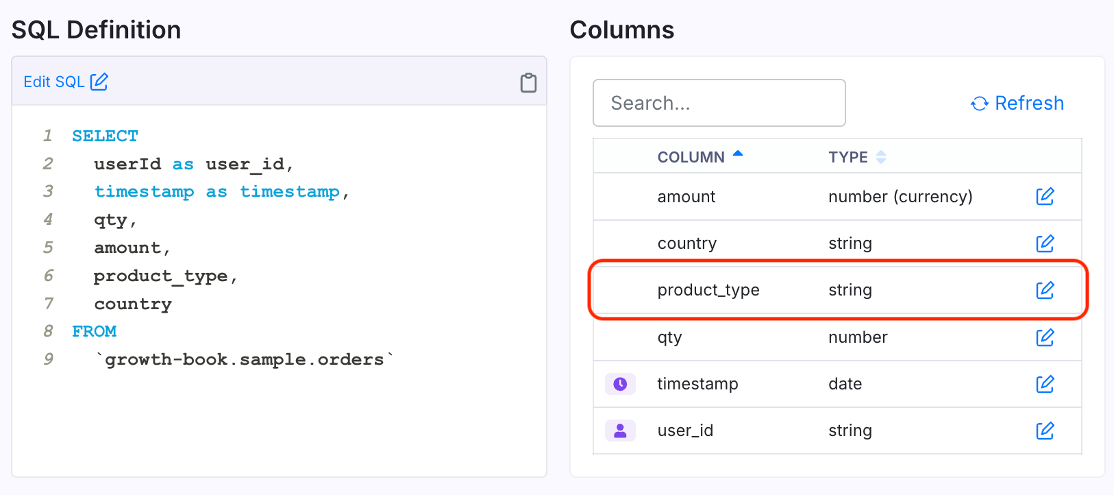
- With your column (
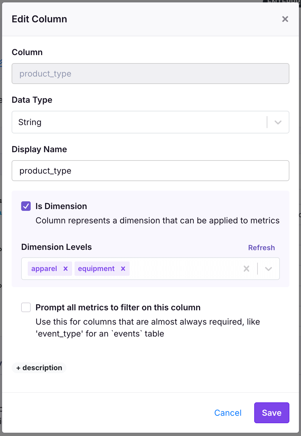
product_type) in the Fact Table SQL, you now edit the column property in the "Columns" table. Click the edit icon next to your column and then check the "Enable Auto Slices" checkbox in the window that pops up.- For string columns, add the slices you want to split your metric by. We run a query to populate the top values for you, and you can update the values found in the data by clicking the "Refresh" button. Slice values here could be "apparel", "equipment", and more. An "other" slice will also be shown if any metric value is attributed to values outside of your selected slices. You can have these levels automatically refresh over time by enabling auto-update slice levels.
- For boolean columns, no other slice configuration is necessary—both "true" and "false" slices will be generated. A "null" slice will also be shown for nullable columns if any metric value is attributed to "null".
- Scroll down to the list of Fact Metrics, or navigate to a Fact Metric from this Fact Table.
- Click "Edit" and select your slices you want to apply to that metric for all experiments.
Auto-update slice levels
You can enable automatic updates of auto slice levels based on top column values. This keeps your slice levels current with your data without manual intervention.
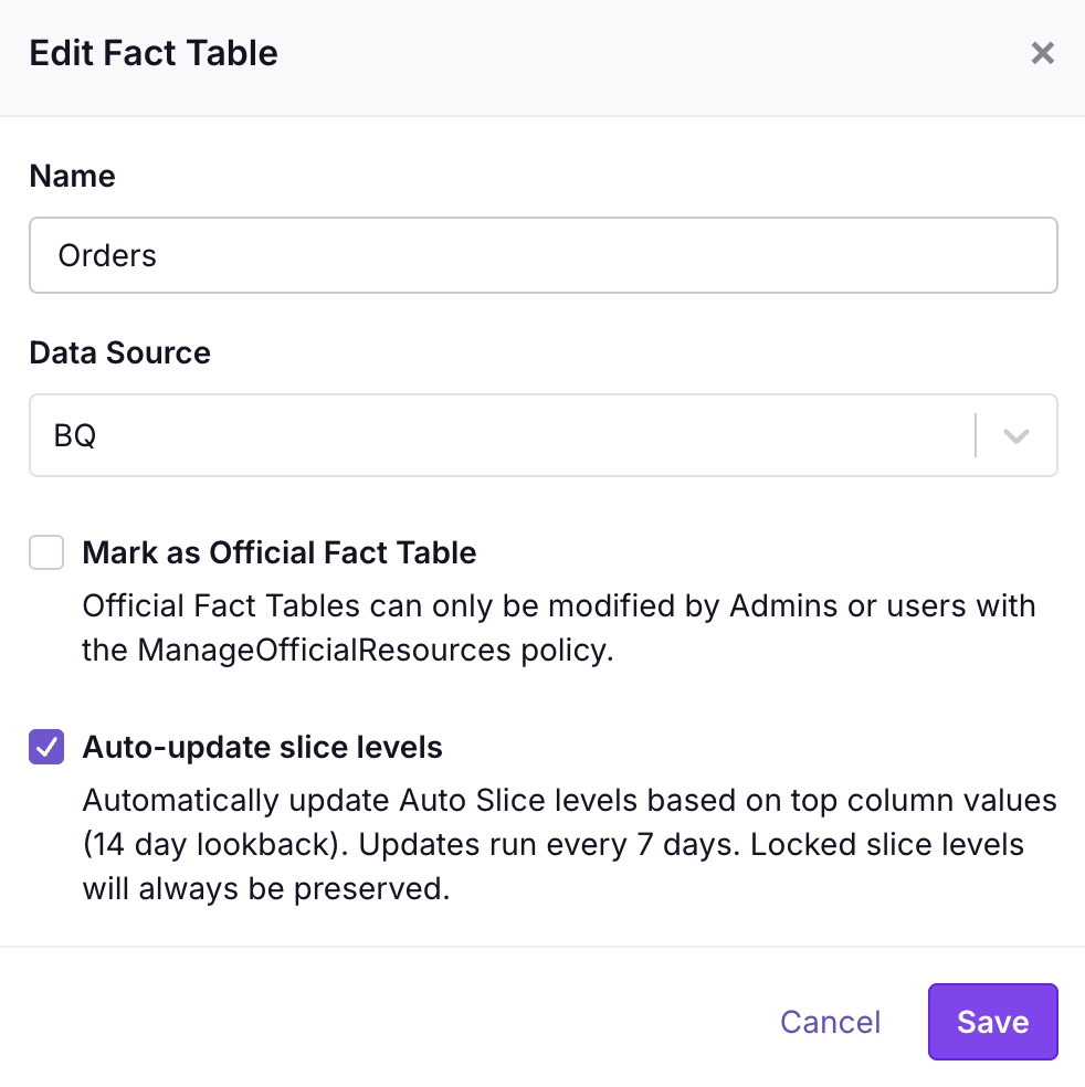
Fact Table level setting:
In the Fact Table modal, check the Auto-update slice levels checkbox. When enabled, a scheduled job periodically refreshes auto slice levels from top values, scanning the lookback window configured in your organization's Data Source settings (default 14 days). The job runs:
- Every 7 days by default (configurable via
AUTO_SLICE_UPDATE_FREQUENCY_HOURSenvironment variable for self-hosted users) - Automatically when the fact table changes
- Manually when you click Update in the column modal
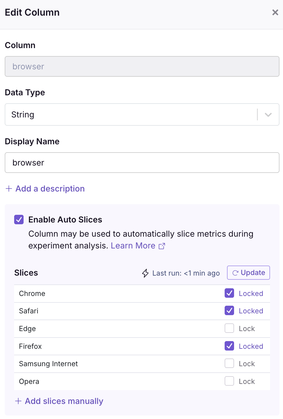
Locking slice levels
When auto-updates are enabled, you can lock specific slice levels in the column modal to ensure they are never removed by the auto-update job. This is useful for important segments or product types that you always want to track, even if they're not currently in the top values.
In the column modal, each slice level has a Lock checkbox. Locked levels are always preserved when the top-values job runs, while unlocked levels may be replaced if they're no longer in the top values.
Custom Slices
We also allow you to perform custom metric breakdowns across all of your experiment metrics for a single experiment. For example: "For this experiment, I want to see how treatment will affect apparel revenue and average order value in EU". Unlike auto slices, custom slices allow you to create filtering combinations from different columns (e.g., product_type = 'apparel' and location = 'EU').
You can add custom slices when setting up your experiment after selecting your metrics, or at any point afterwards. These slices will be run for all metrics in your experiment, but for that experiment only.
Custom slices can be created using any non-user-identifier string or boolean column in your Fact Table. (Custom slicing is not limited to auto-slices columns.)
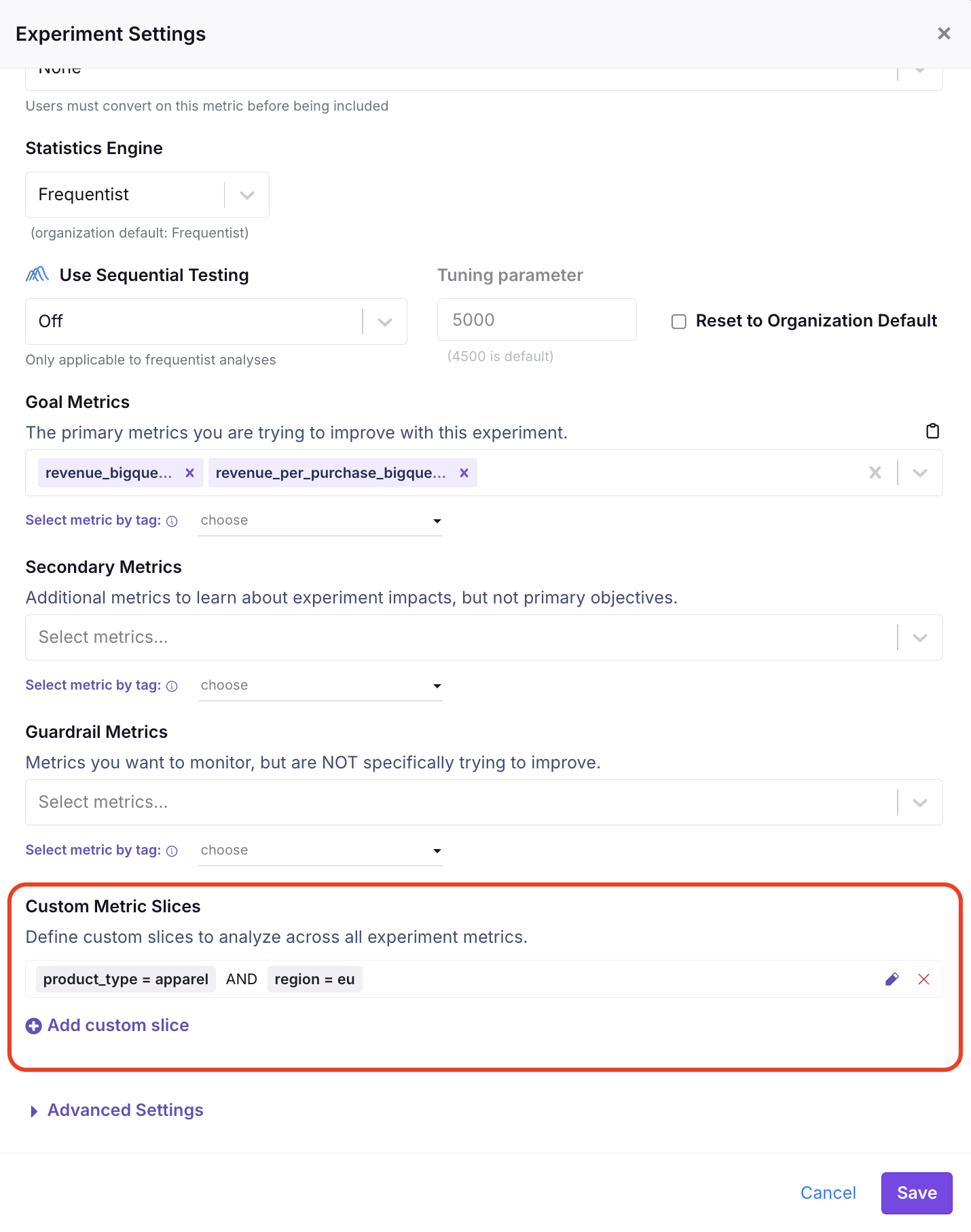
Viewing metric slices
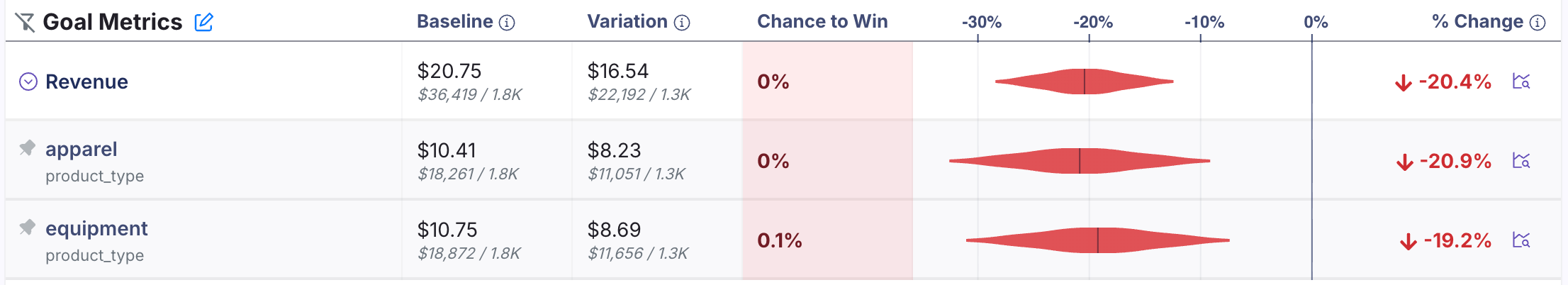
Using our revenue metric as an example, when you run an experiment you will now have the option to split revenue by product type (auto slice) and/or by "apparel and EU" (custom slice).
If you click the arrow icon next to "revenue" on the experiment results table, you will see these slices expand under the base metric row (revenue), each slice materialized as its own sub-row. You also can use the Filter button at the top of the results to filter all metrics by slices, or click in to a row for the Metric Drilldown to view slices with search, sorting, and time-series analysis capabilities.
Unit dimensions and experiment dimensions are attributes specific to an experimental unit (e.g. user). In contrast, metric slices are an attribute specific to a metric. For example, suppose that a user named Romain lives in France, and he buys products from both France and Germany. In a dimension analysis (i.e. a unit dimension analysis), all of Romain's spend will be attributed to France.
In a metric slice analysis, only the French products purchased will be attributed to French revenue, and only the German products purchased will be attributed to German revenue. So one user will always be mapped to a single user dimension, but can contribute to multiple metric slices.
All users (units) contribute to a metric slice. This provides the most accurate inference, as trying to filter down the denominator can cause bias issues if you allow users to switch between different dimension levels.
Metric Analysis
After creating a metric, you can perform some basic analysis on it. Depending on the metric type, we show you the average value over time, a histogram breakdown, and more. You can customize the date range and population that's included.
For more advanced analysis, use our Product Analytics feature.
Metric Groups
EnterpriseMetric Groups is available on Enterprise plans.
There are often groups of metrics you want to add together to an experiment. For example, 5 key revenue metrics that you add to anything touching the checkout flow.
Define Metric Groups to accomplish this. Add multiple metrics, drag & drop to order them, and add them in bulk to experiments as Goals, Guardrails, or Secondary Metrics.
Database Cost Optimization
For large Fact Tables, it can be important to consider query costs, especially when using a data warehouse like BigQuery which charges based on data scanned.
Read our dedicated guide on Query Optimization for best practices on reducing query costs across GrowthBook.