Power

What is power analysis?

Power analysis helps you estimate required experimental duration. Power is the probability of observing a statistically significant result, given your feature has some effect on your metric.

When should I run power analysis?

You should run power analysis before your experiment starts, to determine how long you should run your experiment. The longer the experiment runs, the more users are in the experiment (i.e., your sample size increases). Increasing your sample size lowers the uncertainty around your estimate, which makes it likelier you achieve a statistically significant result.

What is a minimum detectable effect, and how do I interpret it?

The relative effect of your experiment (which we often refer to as simply the effect size) is the percentage improvement in your metric caused by your feature. For example, suppose that average revenue per customer under control is $100, while under treatment you expect that it will be $102. This corresponds to a ($102-$100)/$100 = 2% effect size. Effect size is often referred to as lift.

Given the sample variance of your metric and the sample size, the minimum detectable effect (MDE) is the smallest effect size for which your power will be at least 80%.

GrowthBook includes both power and MDE results to ensure that customers comfortable with either tool can use them to make decisions. The MDE can be thought of as the smallest effect that you will be able to detect most of the time in your experiment. We want to be able to detect subtle changes in metrics, so smaller MDEs are better.

For example, suppose your MDE is 2%. If you feel like your feature could drive a 2% improvement, then your experiment is high-powered. If you feel like your feature will probably only drive something like .5% improvement (which can still be huge!), then you need to add users to reliably detect this effect.

How do I run a power analysis?

1. From the GrowthBook home page, click "Experiments" on the left tab. In the top right, click "Power Calculator."
2. Select “New Calculation”.
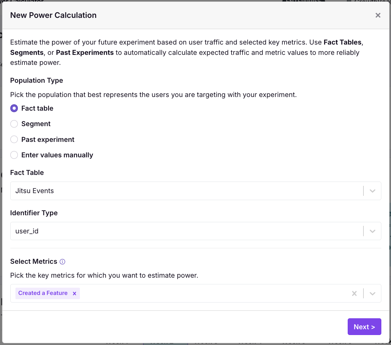
3. On the first page you will select two different components of a power calculation:

• First, the population for your power analysis. This should be the Fact Table, Segment, or Past Experiment that best represents the kind of traffic you will get in the experiment you are planning. We will use this population to estimate both your weekly traffic as well as your metric mean and variance.
• Second, select your goal metrics for your experiment (maximum of 5). Only metrics that can be joined to your population of interest or that were a part of a past experiment can be selected. All non-quantile metrics are supported.

4. On the second page you specify your Expected Effect Size and can customize the traffic and metric values used in the power analysis.

• For each metric, enter the "Expected Effect Size" for each metric. Effect size is the percentage improvement in your metric (i.e., the lift) you anticipate your feature will cause. Inputting your effect size can require care - see here.
• For each metric and for the users per week, we pre-populate the data with values from your selected population, but you can also customize the, if you wish.

5. Now you have results! Please see the results interpretation here.
6. You can modify the number of variations you intend to test, as well as clicking "Edit" in the Analysis Setting box if you want to change your statistics engine or statistics settings.
7. If you want to modify your inputs, click the "Edit" button next to "New Calculation" in the top right corner.

How do I interpret power analysis results?

In this section we run through an example power analysis using our own GrowthBook app (some numbers have been modified for example purposes). For the example, we will use the Jitsu Events fact table as our population. This is basically all users that use GrowthBook regularly, so it mimics an experiment that would happen to all users as they log in to GrowthBook. We will also use the Created a Feature binomial metric, which is 1 for users that create a Feature in 72 hours after the are exposed and 0 otherwise.

When we click next, a query kicks off using the last 8 weeks of data to estimate our expected traffic to this population as well as the metric value.

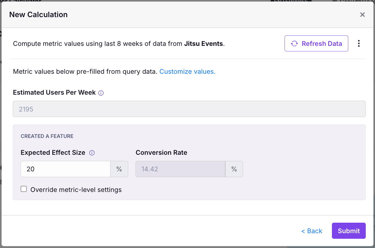
As you can see, the query estimates about 2,195 users per week and a 14.41% of those that Created a Feature in the 72 hours after first appearing in our population (this 72 hour window comes from our metric definition; these kinds of settings on your own metrics will also be applied to make the power calculation more accurate).

We also selected a 20% expected effect size. This is large, but not unattainable based on our past experiments and so it is our best guess for our expected metric improvement. We provide guidance for effect size selection here. For our feature we anticipate a 20% improvement in users creating a feature. We then submit our data.

Now we can see the results!

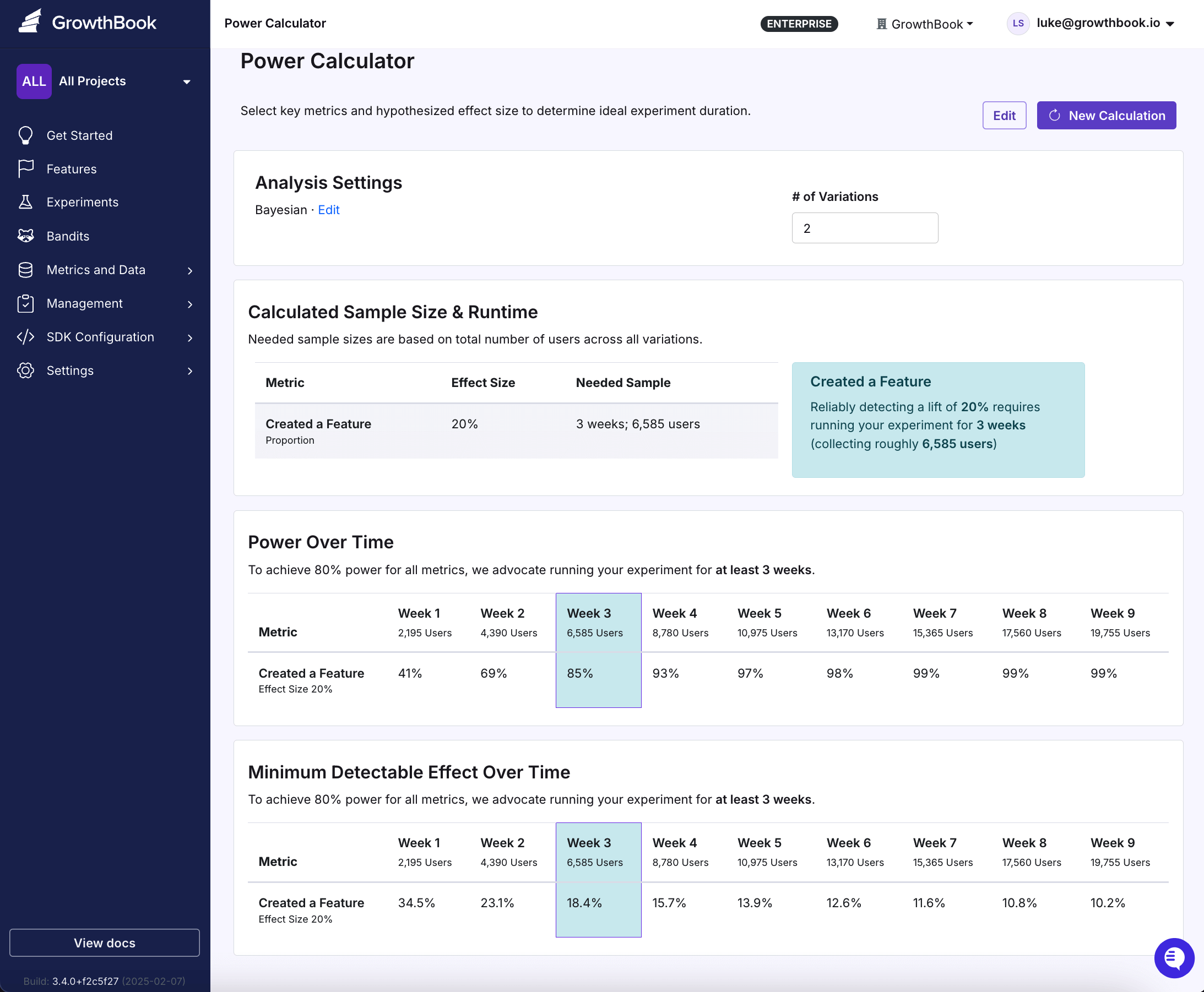
At the top of the page is a box called Analysis Settings. If you want to rerun power results with number of variations greater than 2, then change the "# of Variations" and the results will automatically update. The total traffic divided by number of variations should equal the smallest sample size in the experiment you plan to run. If you want to toggle on or off "Sequential Testing", then press the "Edit" button and select the appropriate option. Enabling sequential testing reduces power.

Below "Analysis Settings" is "Calculated Sample Size and Runtime", which contains the number of weeks (or equivalently the number of users) needed to run your experiment to achieve 80% power by metric. Clicking on a row in the table causes the information in the box to the right to change. We expect 80% power for our binomial metric if we run the experiment for 3 weeks.

Beneath "Calculated Sample Size and Runtime" is "Power Over Time", which contains power estimates by metric. The columns in Power Over Time correspond to different weeks. For example, in the first week power is 41%. The highlighted column in week 3 is the first week where at least 80% power is achieved for our metric. As expected, power increases over time, as new users are added to the experiment.

Beneath Power Over Time is Minimum Detectable Effect Over Time. Minimum Detectable Effect Over Time is structured the same as Power Over Time, except it contains MDEs rather than power estimates. The Week 1 MDE is 34.5%. This means that if your true lift is 34.5%, after 1 week you will have at least 80% chance of observing a statistically significant result. As expected, MDEs decrease over time, as new users are added to the experiment and we have more power to detect smaller and smaller effects.

If you see N/A in your MDE results, this means that you need to increase your number of weekly users, as the MDE calculation failed.

It can be helpful to see power estimates at different effect sizes, different estimates of weekly users, etc. To modify your inputs, click the "Edit" button next to "New Calculation" in the top right corner.

How should I pick my effect size?

Selecting your effect size for power analysis requires careful thought. Your effect size is your anticipated metric lift due to your feature. Obviously you do not have complete information about the true lift, otherwise you would not be running the experiment!

We advocate running power analysis for multiple effect sizes. The following questions may elicit helpful effect sizes:

1. What is your best guess for the potential improvement due to your feature? Are there similar historical experiments, or pilot studies, and if so, what were their lifts?
2. Suppose your feature is amazing - what do you think the lift would be?
3. Suppose your feature impact is smaller than you think - how small could it be?

Ideally your experiment has high power (see here) across a range of effect sizes.

What is a high-powered experiment?

In clinical trials, the standard is 80%. This means that if you were to run your clinical trial 100 times with different patients and different randomizations each time, then you would observe statistically significant results in at least roughly 80 of those trials. When calculating MDEs, we use this default of 80%.

That being said, running an experiment with less than 80% power can still help your business. The purpose of an experiment is to learn about your business, not simply to roll out features that achieve statistically significant improvement. The biggest cost to running low-powered experiments is that your results will be noisy. This usually leads to ambiguity in the rollout decision.

How do I run Bayesian power analysis?

For Bayesian power analysis, you specify the prior distribution of the treatment effect (see here) for guidance regarding prior selection). We then estimate Bayesian power, which is the probability that the $(1 - \alpha)$ credible interval does not contain 0.

If your organizational default is Bayesian, then Bayesian will be your default power analysis. You can switch to and from frequentist and Bayesian power calculations by toggling "Statistics Engine" under "Settings" on the Power Results page.

Your default prior for each metric will be your organizational default. To change a prior for a metric, go to "Settings", and make sure that "Statistics Engine" is toggled to "Bayesian." Then choose "Prior Specification", and update prior means and standard deviations for your metric(s). Remember that these priors are on the relative scale, so a prior mean of 0.1 represents a 10% lift.

FAQ

Frequently asked questions:

1. How can I increase my experimental power? You can increase experimental power by increasing the number of daily users, perhaps by either expanding your population to new segments, or by including a larger percentage of user traffic in your experiment. Similarly, if you have more than 2 variations, reducing the number of variations increases power.
2. What if my experiment is low-powered? Should I still run it? The biggest cost to running a low-powered experiment is that your results will probably be noisy, and you will face ambiguity in your rollout/rollback decision. That being said, you will probably still have learnings from your experiment.
3. What does "N/A" mean for my MDE result? It means there is no solution for the MDE, given the current number of weekly users, control mean, and control variance. Increase your number of weekly users or reduce your number of treatment variations.
4. After looking at my effect estimate and its uncertainty on the GrowthBook UI, I entered them into the power calculator. While my results were statistically significant, the power calculator outputted that my power is less than 80%. Is this an error? This is not an error. Suppose your effect estimate from your experiment is 2%, and it is barely statistically significant. If you enter a 2% effect size into the power calculator (along with the sample means and standard deviations from your results), the power calculator will probably output power less than 80%. Why? Roughly speaking, the power calculator assumes you are going to run 100 experiments in the future. In some of these experiments your estimated effect size will be larger than 2%, and will probably be statistically significant. In others, the estimated effect size will be less than 2%, and may not be statistically significant. If fewer than 80 of these experiments are statistically significant, then your power estimate will be less than 80%. Similarly, if you enter the sample means and standard deviations from your results, the power calculator will probably output and MDE greater than 2%.

GrowthBook implementation

For both Bayesian and frequentist engines, we produce two key estimates:

1. Power - After running the experiment for a given number of weeks and for a hypothesized effect size, what is the probability of a statistically significant result?
2. Minimum Detectable Effect (MDE) - After running an experiment for a given number of weeks, what is the smallest effect that we can detect as statistically significant 80% of the time?

Each engine arrives at these values differently. Below we describe high-level technical details of our implementation. All technical details can be found here.

Frequentist implementation

Below we define frequentist power.

Define:

1. the false positive rate as $\alpha$ (GrowthBook default is $\alpha=0.05$).
2. the critical values $Z_{1- \alpha / 2}= \Phi^{-1}(1-\alpha/2)$ and $Z_{1-\alpha}= \Phi^{-1}(1-\alpha)$ where $\Phi$ is the inverse cumulative distribution function of the standard normal distribution.

We make the following assumptions:

1. equal sample sizes across control and treatment variations. If unequal sample sizes are used in the experiment, use the smaller of the two sample sizes. This will produce conservative power estimates.
2. equal variance across control and treatment variations;
3. observations across users are independent and identically distributed; and
4. all metrics have finite variance.
5. you are running a two-sample t-test. If in practice you use CUPED, your power will be higher. Use CUPED!

For a 2-sided test (all GrowthBook tests are 2-sided), power is the probability of rejecting the null hypothesis of no effect, given that a nonzero effect exists.
Mathematically, frequentist power equals

$$\begin{align} \pi = 1 - \Phi\left(Z_{1-\alpha/2}-\frac{\Delta}{\hat{\sigma}_{\Delta}}\right) + \Phi(Z_{\alpha/2} - \frac{\Delta}{\hat{\sigma}_{\Delta}}). \end{align}$$

Let $HW$ be the interval halfwidth. We can write the above equation as

$$\begin{align} \pi = 1 - \Phi\left( \frac{HW-\Delta}{\hat{\sigma}_{\Delta}} \right) + \Phi\left( \frac{-HW-\Delta}{\hat{\sigma}_{\Delta}} \right) \end{align}$$

The MDE is the smallest effect size for which nominal power (i.e., 80%) is achieved. In the 2-sided case there is no closed form solution. The frequentist MDE is the solution for $\Delta$ when solving for $\pi$ in the equation below:

$\pi = 1 - \Phi\left(Z_{1-\alpha/2}-\frac{\Delta}{\hat{\sigma}_{\Delta}}\right).$

Inverting this equation requires some care, as the uncertainty estimate $\hat{\sigma}_{\Delta}$ depends upon $\Delta$. Details can be found here.

To estimate power under sequential testing, we adjust the variance term $\hat{\sigma}_{\Delta}^{2}$ to account for sequential testing, and then input this adjusted variance into our power formula. We assume that you look at the data only once, so our power estimate below is a lower bound for the actual power under sequential testing. Otherwise we would have to make assumptions about the temporal correlation of the data generating process.

Bayesian implementation

For Bayesian power analysis, we let users specify the prior distribution of the treatment effect (see here for guidance regarding prior selection). We then estimate Bayesian power, which is the probability that the $(1 - \alpha)$ credible interval does not contain 0.

At GrowthBook, Bayesian power is

$$\begin{align} \begin{split} \pi &= 1-\Phi\left( \frac{ \hat{\sigma}_{\Delta}^{2}\left[\left(\frac{1}{\sigma_{prior}^{2}} + \frac{1}{\hat{\sigma}_{\Delta}^{2}}\right)^{1/2} Z_{1-\alpha/2} - \frac{\mu_{prior}}{\sigma_{prior}^{2}}\right]-\Delta} {\sqrt{\hat{\sigma}_{\Delta}^{2}}} \right) \\&+\Phi\left( \frac{ -\hat{\sigma}_{\Delta}^{2}\left[\left(\frac{1}{\sigma_{prior}^{2}} + \frac{1}{\hat{\sigma}_{\Delta}^{2}}\right)^{1/2} Z_{1-\alpha/2} - \frac{\mu_{prior}}{\sigma_{prior}^{2}}\right]-\Delta} {\sqrt{\hat{\sigma}_{\Delta}^{2}}} \right). \end{split} \end{align}$$

Constructing the MDE is less straightforward, as MDEs are not well defined in Bayesian literature. We provide MDEs in Bayesian power analysis for customers that are used to conceptualizing MDEs and want to be able to leverage prior information in their analysis. We define the MDE as the minimum value of $\Delta$ such that at least $\pi$ power is achieved.

The Bayesian MDE is the solution for $\Delta$ when solving for $\pi$ in Equation 1. To find $\Delta$, we use a grid search.