Sequential Testing

note

Sequential Testing is only implemented for the Frequentist statistics engine, and is a premium feature.

Why use sequential testing?

Sequential testing allows you to look at your experiment results as many times as you like while still keeping the number of false positives below the expected rate. In other words, it is the frequentist solution to the peeking problem in AB testing.

Sequential testing not only reduces the risk of false positives in online experimentation; it can also increase the velocity of experimentation. Although sequential testing produces wider confidence intervals than fixed-sample testing, traditional frequentist inference requires an experimenter to wait until a pre-determined sample size is collected. With sequential testing, decisions can be made as soon as significance is reached, without fear of inflating the false positive rate.

The peeking problem

What is peeking? First, some background on frequentist testing.

When running a frequentist analysis, the experimenter sets a confidence level, often written as $\alpha$. Many people, and GrowthBook, default to using $\alpha = 5\%$ (sometimes it is written as $\alpha = 0.05$). These all mean the same thing: for a correctly specified frequentist analysis, you will only reject the null hypothesis 5% of the time when the null hypothesis is true. Usually in online experimentation, our null hypothesis is that metric averages in two variations are the same. In other words, $\alpha$ controls the False Positive Rate.

However, experimenters often violate a fundamental assumption underpinning frequentist analysis: that one must wait until for some pre-specified time (or sample size) before looking at and acting upon experiment results. If you violate this assumption, and peek at your results, you will end up with an inflated False Positive Rate, far above your nominal 5% level. In other words, if we check an experiment as it runs, we are essentially increasing the number of times we can get a positive, even if there is no experiment effect, just through random noise.

We have two options:

1. Stop checking early. This is possible, but in a lot of cases it can make decision making worse! It is powerful to be able to see bad results and shut a feature down early; or conversely to see a great feature do well right away, end the experiment, and ship to everyone.
2. Use an estimator that returns our control over false positive rates.

Sequential testing provides estimators for the second option; it allows peeking at your results without fear of inflating the false positive rate beyond your specified $\alpha$.

Configuring sequential testing

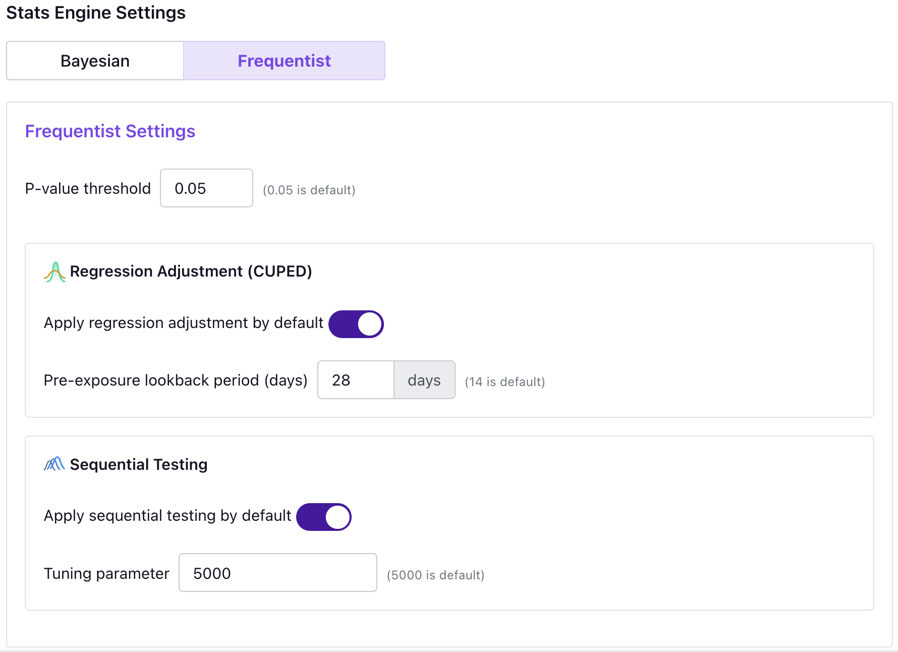
You can enable or disable sequential testing, as well as select your tuning parameter, both in your organization settings (as a default for all future experiments) or on an individual experiment's page.

You can also play with the settings in a custom report.

Setting the tuning parameter

The tuning parameter (written as $N^*$ in the implementation notes below), should be set to the number of observations at which you tend to make decisions. It can be thought of as an "estimated sample size" for the two arms you are comparing. You want to set $N^*$ to be the number of observations at which you tend to make decisions, because it is at that sample size that the loss in experiment power from using sequential testing will be smallest relative to the traditional confidence intervals.

The following figure shows how the increased CI width in sequential analysis is minimized when the sample size is approximately $N^*$. The y-axis is the ratio of the sequential CIs to the regular CIs; all lines are well above 1.0, showing that sequential analysis results in uniformly wider confidence intervals. On the x-axis is the sample size at which the analysis was executed. As you can see, the ratio is lowest when $N^*$ is as close to sample size used in the analysis.

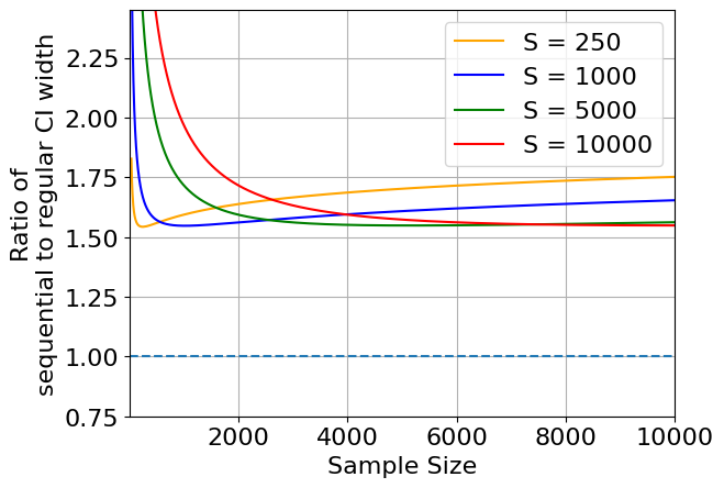
We default to using 5,000, but the general advice is to set this parameter to the sample size you expect to get when you are most likely to make a decision on this experiment. Note, this number reflects the total sample size across the two variations you are comparing. If you have an experiment with 3 variations, and you want the smallest confidence intervals after 3,000 users in each variation, you should set the tuning parameter to 6,000 following the above logic. This is because while the total number of users will be 9,000, there will be 6,000 total in each comparison of arms (e.g. A vs B, B vs C, and A vs C).

Note that the tuning parameter should remain fixed for an experiment.

Organizational defaults

To set the default usage of sequential testing and the tuning parameter for new experiments, navigate to the Organization Settings page and select your preferred defaults.

Experiment settings

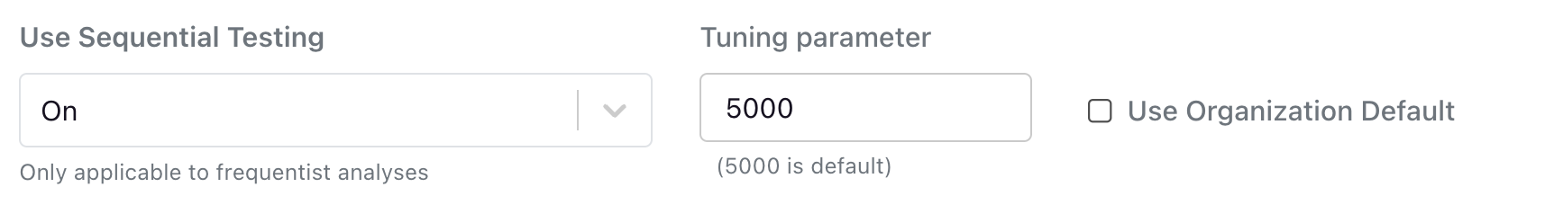
You can also turn sequential testing on and off for an individual experiment, as well as set a specific tuning parameter for that experiment. Navigate to the Experiment page, click Edit Experiment Settings, and choose your preferred settings.

GrowthBook's implementation

There are many approaches to sequential testing, several of which are well explained and compared in this Spotify blogpost.

For GrowthBook, we selected a method that would work for the wide variety of experimenters that we serve, while also providing experimenters with a way to tune the approach for their setting. To that end, we implement Asymptotic Confidence Sequences introduced by Waudby-Smith et al. (2023); these are very similar to the Generalized Anytime Valid Inference confidence sequences described by Spotify in the above post and introduced by Howard et al. (2022), although the Waudby-Smith et al. approach more transparently applies to our setting.

Specifically, GrowthBook's confidence sequences, which take the place of confidence intervals, become:

$\left(\hat{\mu} \pm \hat{\sigma}*\sqrt{N}*\sqrt{\frac{2(N\rho^2 + 1)}{N^{2}\rho^2}\log\left(\frac{\sqrt{N\rho^2 + 1}}{\alpha}\right)}\right)$

$\rho = \sqrt{\frac{-2\text{log}(\alpha) + \text{log}(-2 \text{log}(\alpha) + 1)}{N^*}}$

In the above, $\hat{\mu}$ is our estimated uplift, $\hat{\sigma}$ is the estimated standard error of the uplift, $\alpha$ is our significance level (defaults to 0.05), and $N$ is the sum of the two variation's sample sizes.

In the above $N^*$ is a tuning parameter that lets us control how tight these confidence sequences are relative to the standard, fixed-time confidence intervals. You can read more about how to set it in the Configuring Sequential Testing section.